Last updated: 2020-07-21

Checks: 5 2

Knit directory: psychencode/

This reproducible R Markdown analysis was created with workflowr (version 1.6.2). The Checks tab describes the reproducibility checks that were applied when the results were created. The Past versions tab lists the development history.

R Markdown file: uncommitted changes

The R Markdown is untracked by Git. To know which version of the R Markdown file created these results, you’ll want to first commit it to the Git repo. If you’re still working on the analysis, you can ignore this warning. When you’re finished, you can run wflow_publish to commit the R Markdown file and build the HTML.

Environment: empty

Great job! The global environment was empty. Objects defined in the global environment can affect the analysis in your R Markdown file in unknown ways. For reproduciblity it’s best to always run the code in an empty environment.

Seed: set.seed(20200622)

The command set.seed(20200622) was run prior to running the code in the R Markdown file. Setting a seed ensures that any results that rely on randomness, e.g. subsampling or permutations, are reproducible.

Session information: recorded

Great job! Recording the operating system, R version, and package versions is critical for reproducibility.

Cache: none

Nice! There were no cached chunks for this analysis, so you can be confident that you successfully produced the results during this run.

File paths: absolute

Using absolute paths to the files within your workflowr project makes it difficult for you and others to run your code on a different machine. Change the absolute path(s) below to the suggested relative path(s) to make your code more reproducible.

absolute	relative
/Users/sabrinami/Github/psychencode	.

Repository version: f161714

Great! You are using Git for version control. Tracking code development and connecting the code version to the results is critical for reproducibility.

The results in this page were generated with repository version f161714. See the Past versions tab to see a history of the changes made to the R Markdown and HTML files.

Note that you need to be careful to ensure that all relevant files for the analysis have been committed to Git prior to generating the results (you can use wflow_publish or wflow_git_commit). workflowr only checks the R Markdown file, but you know if there are other scripts or data files that it depends on. Below is the status of the Git repository when the results were generated:


Ignored files:
    Ignored:    .DS_Store
    Ignored:    .Rhistory
    Ignored:    .Rproj.user/
    Ignored:    analysis/.DS_Store
    Ignored:    output/.DS_Store

Untracked files:
    Untracked:  analysis/test_scz_clozuk_pgc.Rmd
    Untracked:  models/
    Untracked:  output/test_results/

Note that any generated files, e.g. HTML, png, CSS, etc., are not included in this status report because it is ok for generated content to have uncommitted changes.

There are no past versions. Publish this analysis with wflow_publish() to start tracking its development.

We are testing our prediction model derived from a PsychENCODE TWAS, by comparing its S-PrediXcan association results with GTEx Brain Cortex and Whole Blood tissue models. We are using the Walters Group Schizophrenia GWAS. # Definitions

conda activate imlabtools
METAXCAN=/Users/sabrinami/Github/MetaXcan/software
MODEL=/Users/sabrinami/Github/psychencode/models
RESULTS=/Users/sabrinami/Github/psychencode/output/test_results
DATA=/Users/sabrinami/Desktop/psychencode_test_data

Similarly, in R, load the libraries, then set the same definitions.

suppressPackageStartupMessages(library(tidyverse))
suppressPackageStartupMessages(library(qqman))
suppressPackageStartupMessages(library(data.table))
suppressPackageStartupMessages(library(RSQLite))
suppressPackageStartupMessages(library(UpSetR))

PRE="/Users/sabrinami/Github/psychencode"
DATA="/Users/sabrinami/Desktop/psychencode_test_data"
RESULTS=glue::glue("{PRE}/output/test_results")
CODE=glue::glue("{PRE}/code")
MODEL=glue::glue("{PRE}/models")
source(glue::glue("{CODE}/load_data_functions.R"))
source(glue::glue("{CODE}/plotting_utils_functions.R"))

gencode_df = load_gencode_df()

Download Data

The Walters Group in the Psychiatric Genomics Consortium released a Schizophrenia GWAS, from genome-wide genotype data from the UK (CLOZUK sample) and the PGC. There were 40,675 cases and 64,643 controls in the combined analysis. More info on the study: https://www.nature.com/articles/s41588-018-0059-2#MOESM4 More info on the GWAS results: https://walters.psycm.cf.ac.uk To download the data, run.

cd $DATA
wget "https://walters.psycm.cf.ac.uk/clozuk_pgc2.meta.sumstats.txt.gz" --no-check-certificate
gunzip clozuk_pgc2.meta.sumstats.txt.gz

Reformatting

The snps in the GWAS are in IMPUTE2 format, so it will need to be modified to match the prediction models’ varID format. ## Load GWAS and Plot First, we plot the GWAS.

scz_GWAS = fread(glue::glue("{DATA}/clozuk_pgc2.meta.sumstats.txt.gz"), header=TRUE, sep="\t")
# manhattan(scz_GWAS, chr="CHR", bp="BP", snp="SNP", p="P" )
# gg_qqplot(scz_GWAS$P)

Reformat GWAS

Modify the SNPS column to match model format, chr_pos_ref_alt_build. The varID column matches the psychencode model varID format, and varID_v7 will match GTEx v7.

scz_GWAS_mod <- scz_GWAS %>% mutate(A1=toupper(A1), A2=toupper(A2), varID = paste(paste("chr", CHR, sep=""), BP, A1, A2, "b37", sep="_"), varID_v7 = paste(CHR, BP, A1, A2, "b37", sep="_"))
write.table(scz_GWAS_mod, glue::glue("{DATA}/clozuk_pgc2.meta.sumstats.out.txt"), quote=FALSE, row.names=FALSE, sep = "\t")

Reformat Model Covariance

The GWAS is missing rsids, so the varIDs will be used to match snps in the GWAS to those in the models. The covariance files use rsids, which should be replaced with their varIDs. The weights table in the model has the rsid and varID for each snp, so this mapping can be used to swap in the covariance matrix. First, open a connection to the model, then query the weights table. Load the covariance matrix.

psychencode_model = glue::glue("{MODEL}/psychencode_model/psychencode.db")
conn <- dbConnect(RSQLite::SQLite(), psychencode_model)
snps <- dbGetQuery(conn, 'SELECT rsid, varID FROM weights')
snps_mapping <- distinct(snps)
dbDisconnect(conn)

Define the varId-rsid snp mapping using the unique snps in the weights table. Replace the RSID1 and RSID2 columns with left joins, then save the table.

psychencode_covariance = fread(glue::glue("{MODEL}/psychencode_model/psychencode.txt.gz"), header=TRUE, sep=" ")
psychencode_covariance_mod <- psychencode_covariance %>% left_join(snps_mapping, by=c("RSID1"="rsid")) %>% select(GENE, varID, RSID2, VALUE) %>% rename(RSID1 = varID)
psychencode_covariance_mod <- psychencode_covariance_mod %>% left_join(snps_mapping, by=c("RSID2"="rsid")) %>% select(GENE, RSID1, varID, VALUE) %>% rename(RSID2 = varID)
write.table(psychencode_covariance_mod, glue::glue("{MODEL}/psychencode_model/psychencode_varID.txt"), quote=FALSE, row.names=FALSE)

Repeat for the GTEx models.

Brain_Cortex_model = glue::glue("{MODEL}/GTEx-V7-en/gtex_v7_Brain_Cortex_imputed_europeans_tw_0.5_signif.db")
conn <- dbConnect(RSQLite::SQLite(), Brain_Cortex_model)
snps <- dbGetQuery(conn, 'SELECT rsid, varID FROM weights')
snps_mapping <- distinct(snps)
dbDisconnect(conn)

Brain_Cortex_covariance = fread(glue::glue("{MODEL}/GTEx-V7-en/gtex_v7_Brain_Cortex_imputed_eur_covariances.txt.gz"), header=TRUE, sep=" ")
Brain_Cortex_covariance_mod <- Brain_Cortex_covariance %>% left_join(snps_mapping, by=c("RSID1"="rsid")) %>% select(GENE, varID, RSID2, VALUE) %>% rename(RSID1 = varID)
Brain_Cortex_covariance_mod <- Brain_Cortex_covariance_mod %>% left_join(snps_mapping, by=c("RSID2"="rsid")) %>% select(GENE, RSID1, varID, VALUE) %>% rename(RSID2 = varID)
write.table(Brain_Cortex_covariance_mod, glue::glue("{MODEL}/GTEx-V7-en/gtex_v7_Brain_Cortex_imputed_eur_covariances_varID.txt"), quote=FALSE, row.names=FALSE)

Whole_Blood_model = glue::glue("{MODEL}/GTEx-V7-en/gtex_v7_Whole_Blood_imputed_europeans_tw_0.5_signif.db")
conn <- dbConnect(RSQLite::SQLite(), Whole_Blood_model)
snps <- dbGetQuery(conn, 'SELECT rsid, varID FROM weights')
snps_mapping <- distinct(snps)
dbDisconnect(conn)

Whole_Blood_covariance = fread(glue::glue("{MODEL}/GTEx-V7-en/gtex_v7_Whole_Blood_imputed_eur_covariances.txt.gz"), header=TRUE, sep=" ")
Whole_Blood_covariance_mod <- Whole_Blood_covariance %>% left_join(snps_mapping, by=c("RSID1"="rsid")) %>% select(GENE, varID, RSID2, VALUE) %>% rename(RSID1 = varID)
Whole_Blood_covariance_mod <- Whole_Blood_covariance_mod %>% left_join(snps_mapping, by=c("RSID2"="rsid")) %>% select(GENE, RSID1, varID, VALUE) %>% rename(RSID2 = varID)
write.table(Whole_Blood_covariance_mod, glue::glue("{MODEL}/GTEx-V7-en/gtex_v7_Whole_Blood_imputed_eur_covariances_varID.txt"), quote=FALSE, row.names=FALSE)

Lastly, compress the new covariances files.

gzip $MODEL/psychencode_model/psychencode_varID.txt
gzip $MODEL/GTEx-V7-en/gtex_v7_Brain_Cortex_imputed_eur_covariances_varID.txt
gzip $MODEL/GTEx-V7-en/gtex_v7_Whole_Blood_imputed_eur_covariances_varID.txt

Run S-PrediXcan

Run S-PrediXcan on SCZ GWAS with psychencode model, and repeat for GTEx Brain Cortex and Whole Blood models. This used the varIDs instead of rsids to match snps in the GWAS and the models.

python3 $METAXCAN/SPrediXcan.py --gwas_file $DATA/clozuk_pgc2.meta.sumstats.out.txt \
--model_db_path $MODEL/psychencode_model/psychencode.db \
--covariance $MODEL/psychencode_model/psychencode_varID.txt.gz \
--keep_non_rsid --model_db_snp_key varID \
--or_column OR \
--pvalue_column P \
--snp_column varID \
--non_effect_allele_column A2 \
--effect_allele_column A1 \
--throw \
--output_file $RESULTS/spredixcan/eqtl/clozuk_pgc2/clozuk_pgc2_psychencode.csv

Repeat for GTEx models.

python3 $METAXCAN/SPrediXcan.py --gwas_file $DATA/clozuk_pgc2.meta.sumstats.out.txt \
--model_db_path $MODEL/GTEx-V7-en/gtex_v7_Brain_Cortex_imputed_europeans_tw_0.5_signif.db \
--covariance $MODEL/GTEx-V7-en/gtex_v7_Brain_Cortex_imputed_eur_covariances_varID.txt.gz \
--keep_non_rsid --remove_ens_version --model_db_snp_key varID \
--or_column OR \
--pvalue_column P \
--snp_column varID_v7 \
--non_effect_allele_column A2 \
--effect_allele_column A1 \
--throw \
--output_file $RESULTS/spredixcan/eqtl/clozuk_pgc2/clozuk_pgc2_Brain_Cortex.csv

python3 $METAXCAN/SPrediXcan.py --gwas_file $DATA/clozuk_pgc2.meta.sumstats.out.txt \
--model_db_path $MODEL/GTEx-V7-en/gtex_v7_Whole_Blood_imputed_europeans_tw_0.5_signif.db \
--covariance $MODEL/GTEx-V7-en/gtex_v7_Whole_Blood_imputed_eur_covariances_varID.txt.gz \
--keep_non_rsid --additional_output --model_db_snp_key varID \
--or_column OR \
--pvalue_column P \
--snp_column varID_v7 \
--non_effect_allele_column A2 \
--effect_allele_column A1 \
--throw \
--output_file $RESULTS/spredixcan/eqtl/clozuk_pgc2/clozuk_pgc2_Whole_Blood.csv

S-PrediXcan Results

Load the psychencode S-PrediXcan association results, and check for significant genes.

spredixcan_association_psychencode = load_spredixcan_association(glue::glue("{RESULTS}/spredixcan/eqtl/clozuk_pgc2/clozuk_pgc2_psychencode.csv"), gencode_df)
dim(spredixcan_association_psychencode)

[1] 14021    14

significant_genes_psychencode <- spredixcan_association_psychencode %>% filter(pvalue < 0.05/nrow(spredixcan_association_psychencode)) %>% arrange(pvalue)

Repeat for GTEx models.

spredixcan_association_Brain_Cortex = load_spredixcan_association(glue::glue("{RESULTS}/spredixcan/eqtl/clozuk_pgc2/clozuk_pgc2_Brain_Cortex.csv"), gencode_df)
dim(spredixcan_association_Brain_Cortex)

[1] 4246   14

significant_genes_Brain_Cortex <- spredixcan_association_Brain_Cortex %>% filter(pvalue < 0.05/nrow(spredixcan_association_Brain_Cortex)) %>% arrange(pvalue)

spredixcan_association_Whole_Blood = load_spredixcan_association(glue::glue("{RESULTS}/spredixcan/eqtl/clozuk_pgc2/clozuk_pgc2_Whole_Blood.csv"), gencode_df)
dim(spredixcan_association_Whole_Blood)

[1] 6161   16

significant_genes_Whole_Blood <- spredixcan_association_Whole_Blood %>% filter(pvalue < 0.05/nrow(spredixcan_association_Whole_Blood)) %>% arrange(pvalue)

Plot S-PrediXcan Association

For each of the models, we can make a histogram and Q-Q plot of the genes with their p-values, which confirm that all three find significant genes.

significant_genes <- list(Brain_Cortex = significant_genes_Brain_Cortex$gene,
              Whole_Blood = significant_genes_Whole_Blood$gene,
              Psychencode = significant_genes_psychencode$gene)
upset(fromList(significant_genes), order.by = 'freq', empty.intersections = 'on')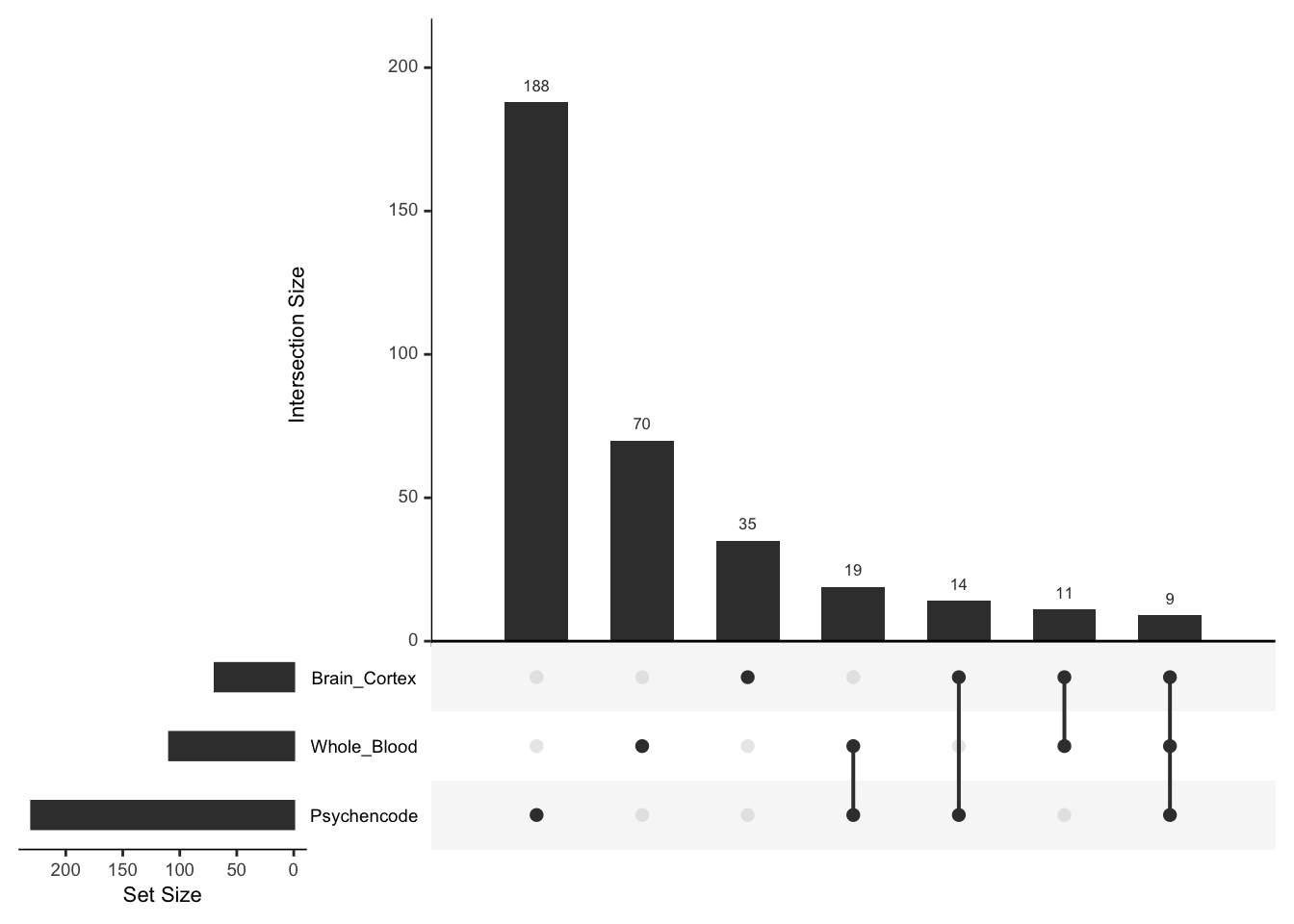

However, Q-Q plots show that all three models have significant genes. For each of the models, we can make a histogram and Q-Q plot of the genes with their p-values.

spredixcan_association_psychencode %>% arrange(pvalue) %>% ggplot(aes(pvalue)) + geom_histogram(bins=20)

Warning: Removed 30 rows containing non-finite values (stat_bin).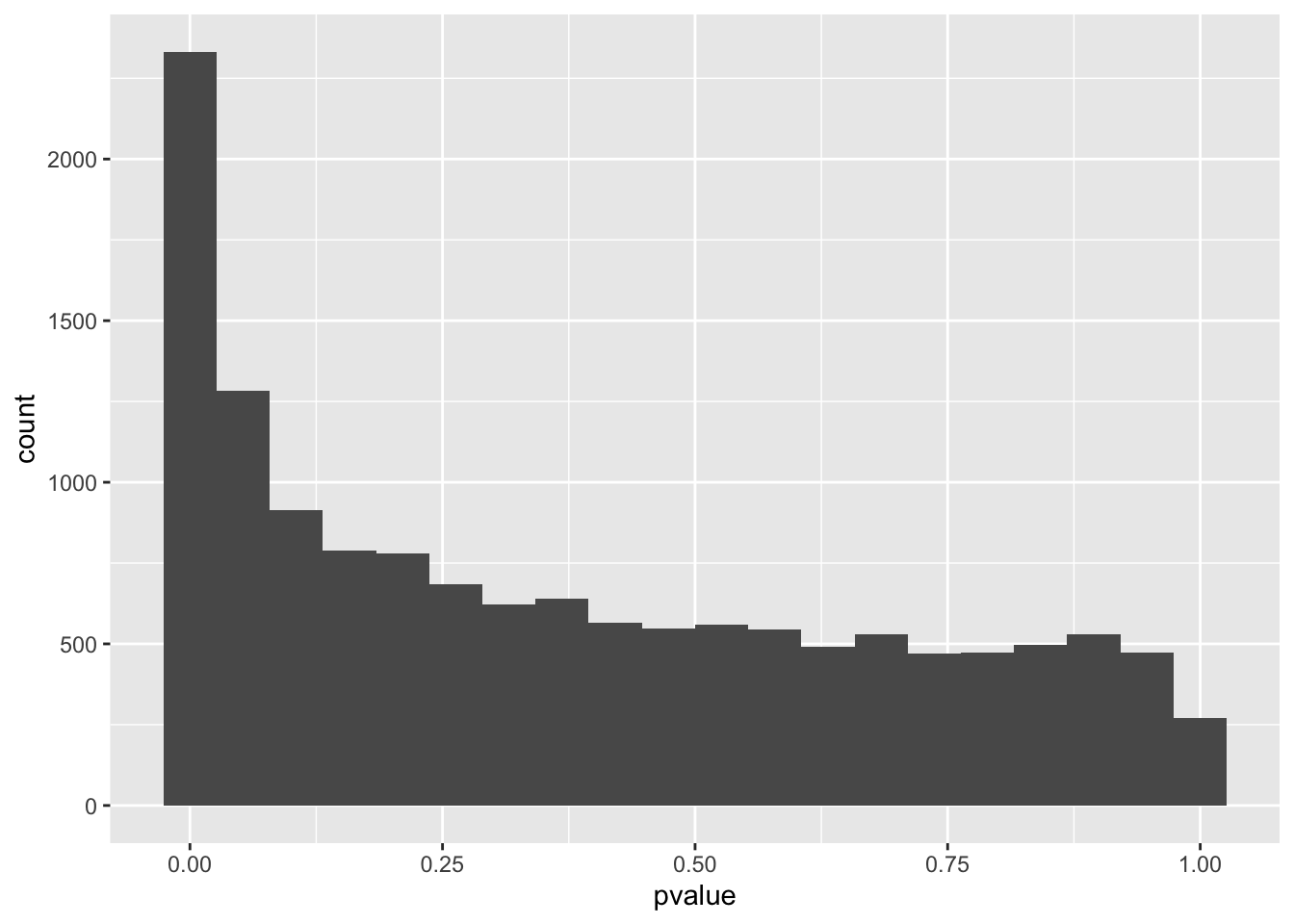

gg_qqplot(spredixcan_association_psychencode$pvalue)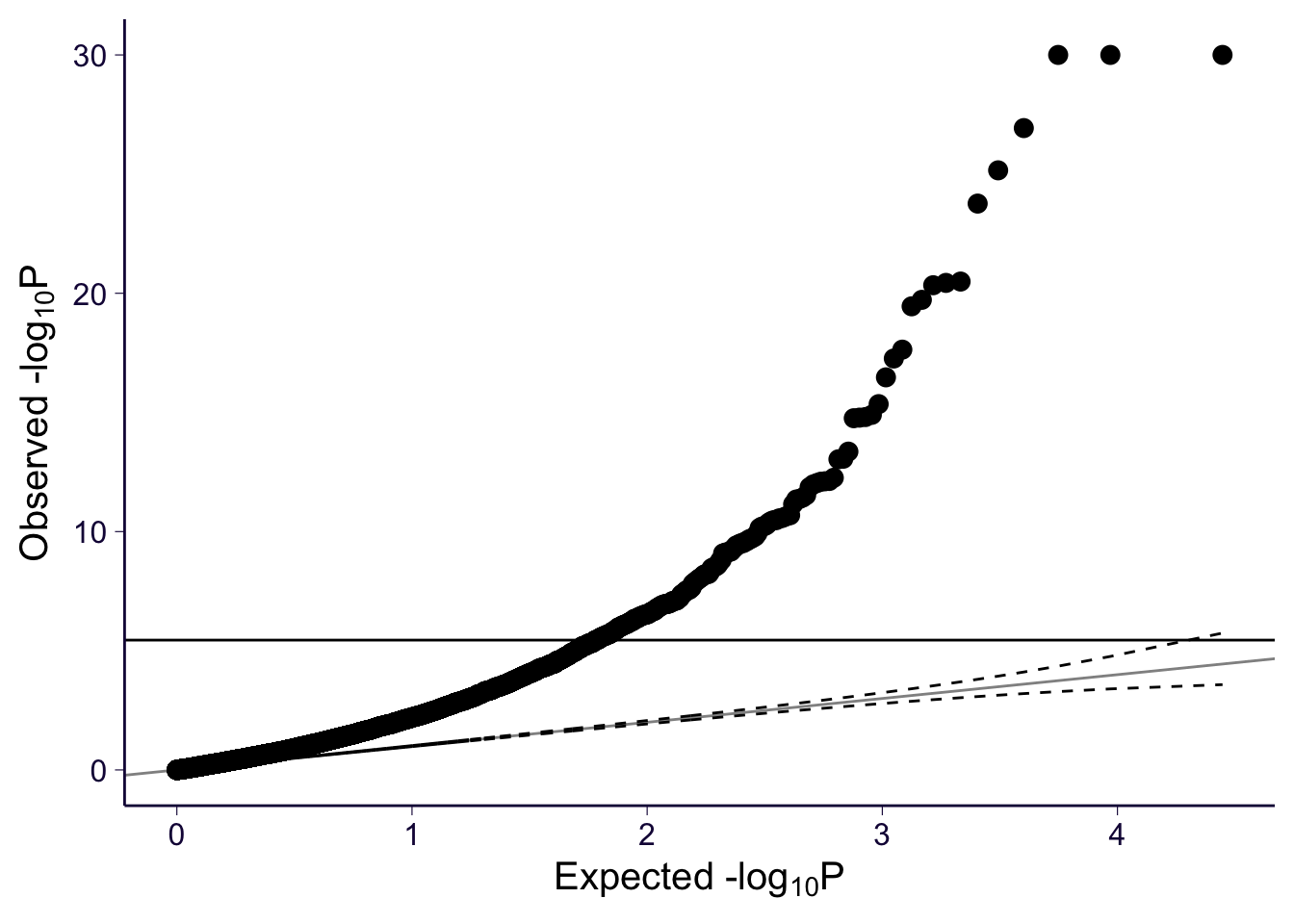

spredixcan_association_Brain_Cortex %>% arrange(pvalue) %>% ggplot(aes(pvalue)) + geom_histogram(bins=20)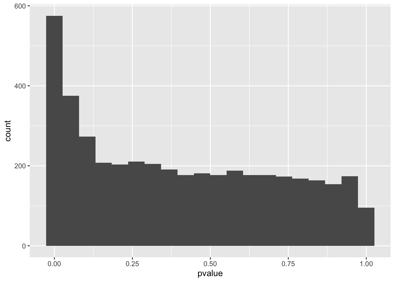

gg_qqplot(spredixcan_association_Brain_Cortex$pvalue)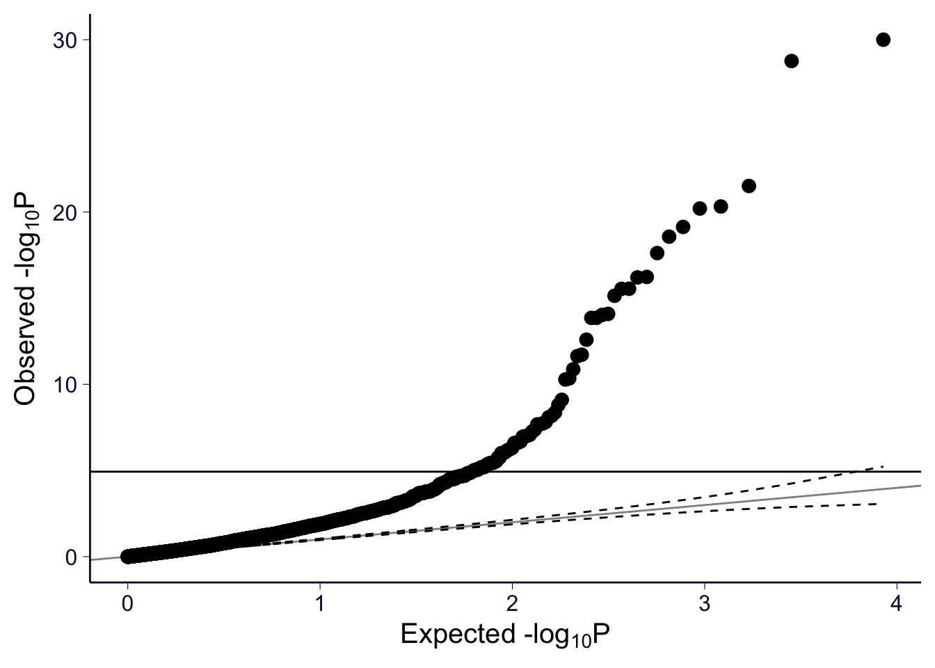

spredixcan_association_Whole_Blood %>% arrange(pvalue) %>% ggplot(aes(pvalue)) + geom_histogram(bins=20)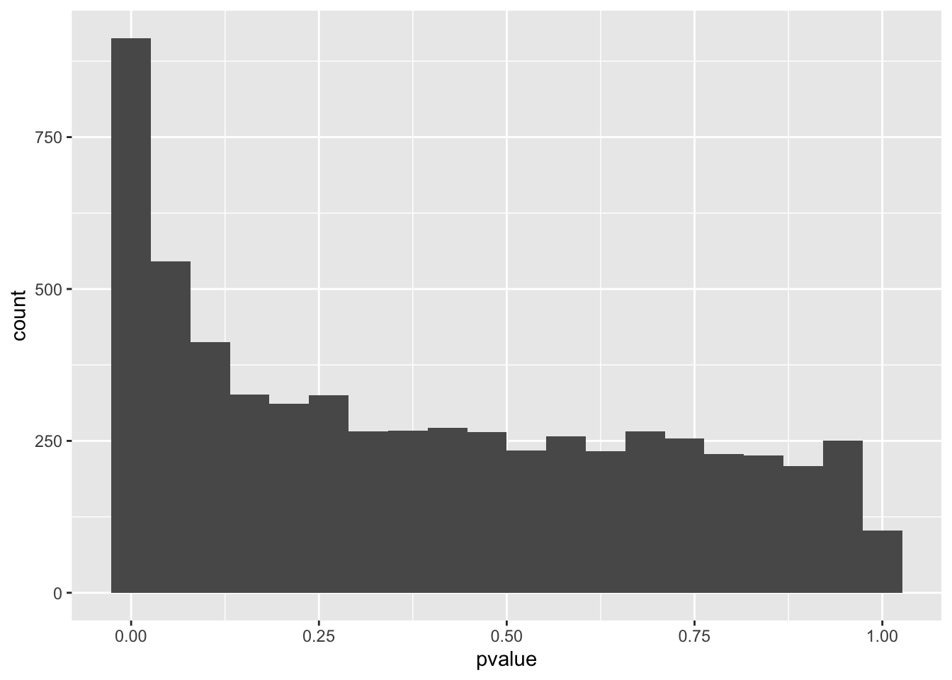

gg_qqplot(spredixcan_association_Whole_Blood$pvalue)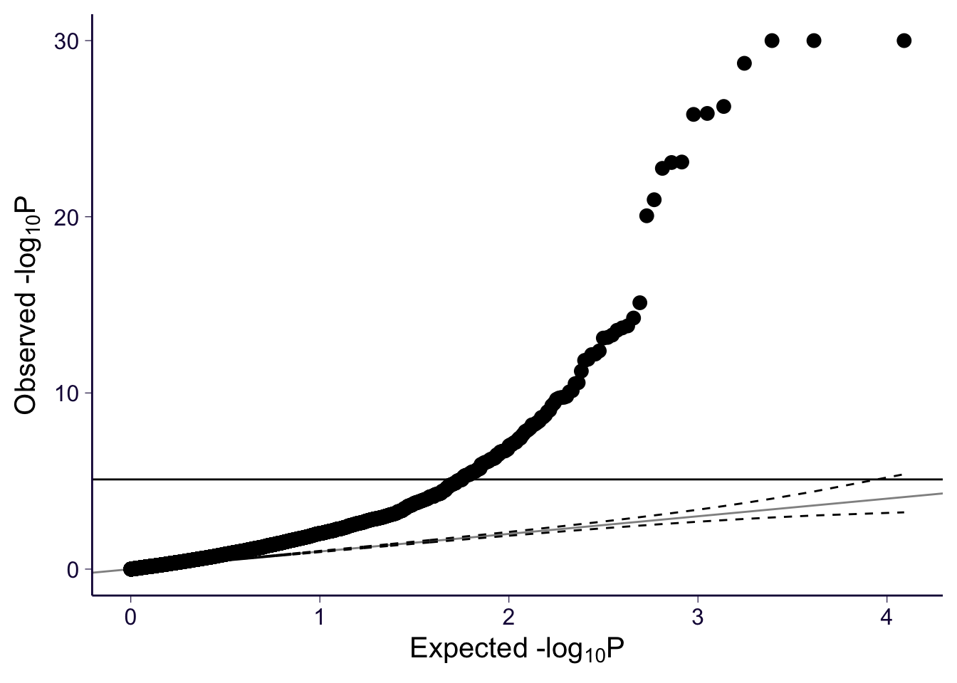

Next, we can plot the distribution of z-scores for each model:

zscore_psychencode <- data.frame("zscore" = spredixcan_association_psychencode$zscore, "model" = "psychENCODE")
zscore_Brain_Cortex <- data.frame("zscore" = spredixcan_association_Brain_Cortex$zscore, "model" = "Brain Cortex")
zscore_Whole_Blood <- data.frame("zscore" = spredixcan_association_Whole_Blood$zscore, "model" = "Whole Blood")
zscore <- rbind(zscore_Brain_Cortex, zscore_psychencode, zscore_Whole_Blood)
ggplot(zscore, aes(x=model, y= zscore)) + geom_violin() + geom_boxplot(width=.4) + ggtitle("Distribution of Association Z-score")

Warning: Removed 30 rows containing non-finite values (stat_ydensity).

Warning: Removed 30 rows containing non-finite values (stat_boxplot).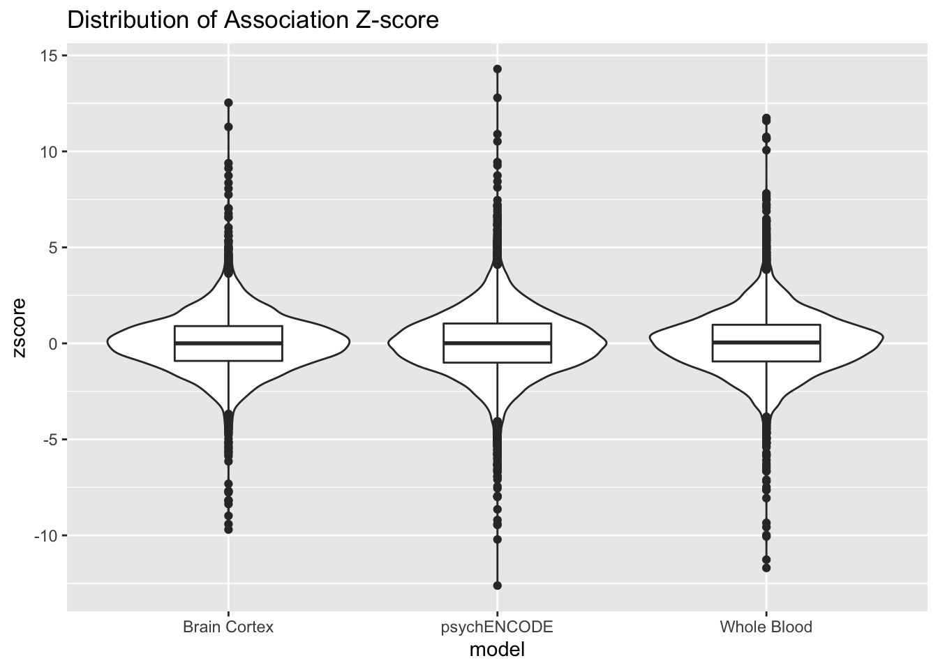

We also compare z-scores between each model. Ideally, the z-scores calculated from multiple model are similar for each gene, so they would follow the identity line. First, plot the Brain Cortex and Psychencode z-scores:

Brain_Cortex_psychencode_zscores = inner_join(spredixcan_association_Brain_Cortex, spredixcan_association_psychencode, by=c("gene"))
dim(Brain_Cortex_psychencode_zscores)

[1] 3339   27

Brain_Cortex_psychencode_zscores %>% ggplot(aes(zscore.x, zscore.y)) + geom_point() + ggtitle("S-PrediXcan z-score") + xlab("GTex Brain Cortex") + ylab("PsychENCODE") + geom_abline(intercept = 0, slope = 1)

Warning: Removed 6 rows containing missing values (geom_point).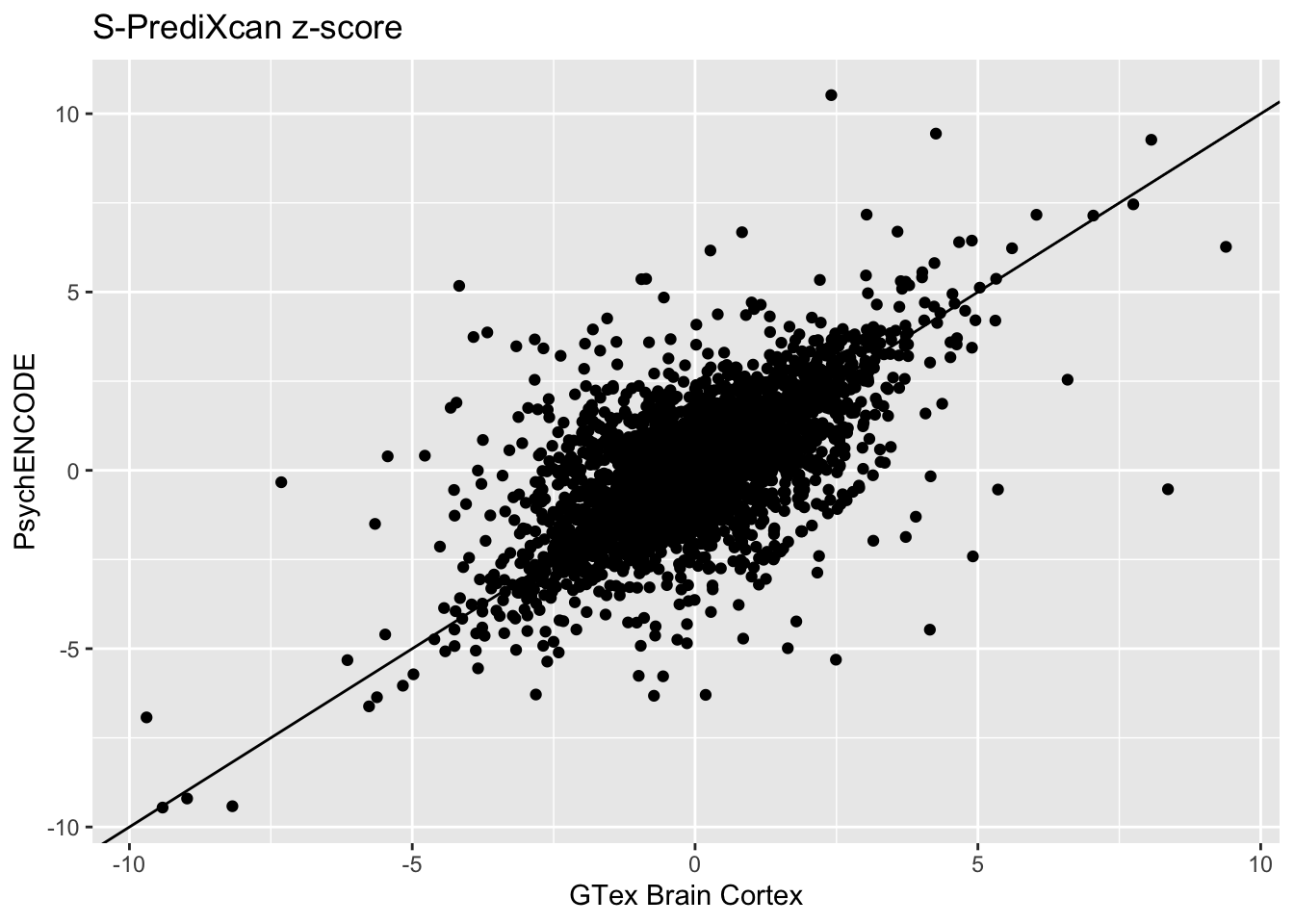

Whole Blood and Psychencode:

Whole_Blood_psychencode_zscores = inner_join(spredixcan_association_Whole_Blood, spredixcan_association_psychencode, by=c("gene"))
dim(Whole_Blood_psychencode_zscores)

[1] 4215   29

Whole_Blood_psychencode_zscores %>% ggplot(aes(zscore.x, zscore.y)) + geom_point() + ggtitle("S-PrediXcan z-score") + xlab("GTex Whole Blood") + ylab("PsychENCODE") + geom_abline(intercept = 0, slope = 1)

Warning: Removed 11 rows containing missing values (geom_point).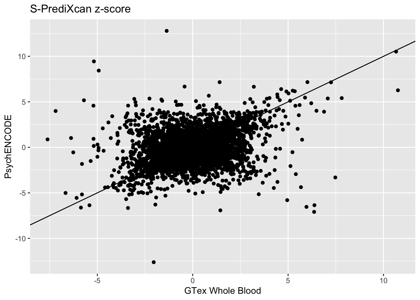

Whole Blood and Brain Cortex:

Whole_Blood_Brain_Cortex_zscores = inner_join(spredixcan_association_Whole_Blood, spredixcan_association_Brain_Cortex, by=c("gene"))
dim(Whole_Blood_Brain_Cortex_zscores)

[1] 1908   29

Whole_Blood_Brain_Cortex_zscores %>% ggplot(aes(zscore.x, zscore.y)) + geom_point() + ggtitle("S-PrediXcan z-score") + xlab("GTex Whole Blood") + ylab("GTEx Brain Cortex") + geom_abline(intercept = 0, slope = 1)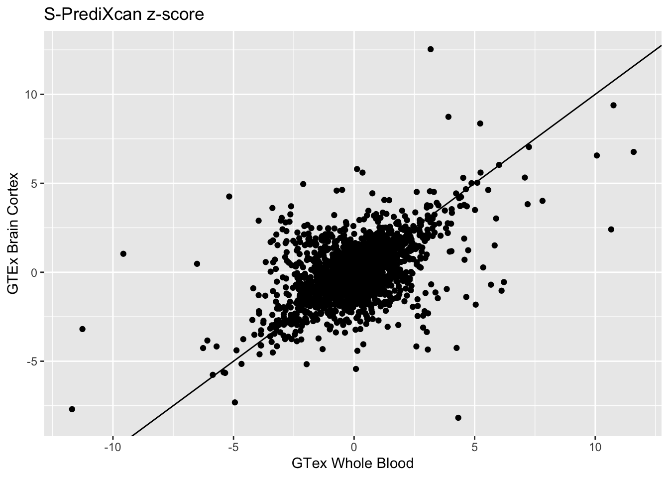

As a sanity check, we can also compare the association results from the PGC GWAS and CLOZUK+PGC GWAS.

spredixcan_association_psychencode2 = load_spredixcan_association(glue::glue("{RESULTS}/spredixcan/eqtl/pgc_scz/SCZvsCONT_psychencode.csv"), gencode_df)
dim(spredixcan_association_psychencode2)

[1] 14320    14

significant_genes_psychencode2 <- spredixcan_association_psychencode2 %>% filter(pvalue < 0.05/nrow(spredixcan_association_psychencode2)) %>% arrange(pvalue)

significant_genes_scz <- list(PsychENCODE_PGC =
                            significant_genes_psychencode2$gene,
                          PsychENCODE_CLOZUK_PGC=
                            significant_genes_psychencode$gene)
upset(fromList(significant_genes_scz), order.by = 'freq', empty.intersections = 'on')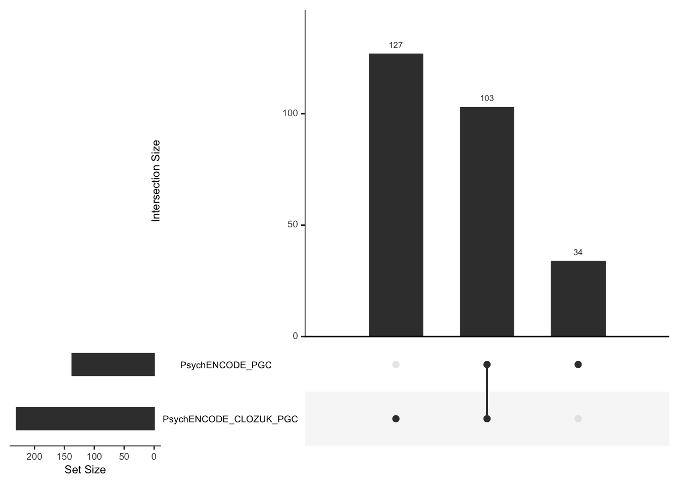

psychencode_zscores = inner_join(spredixcan_association_psychencode2, spredixcan_association_psychencode, by=c("gene"))
dim(psychencode_zscores)

[1] 13992    27

psychencode_zscores %>% ggplot(aes(zscore.x, zscore.y)) + geom_point() + ggtitle("S-PrediXcan z-score") + xlab("PsychENCODE PGC") + ylab("PsychENCODE PGC+CLOZUK") + geom_abline(intercept = 0, slope = 1)

Warning: Removed 32 rows containing missing values (geom_point).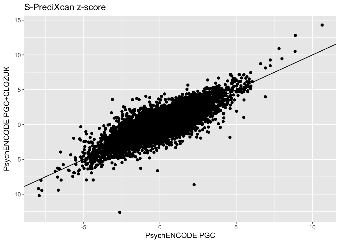

sessionInfo()

R version 3.6.2 (2019-12-12)
Platform: x86_64-apple-darwin15.6.0 (64-bit)
Running under: macOS Mojave 10.14.6

Matrix products: default
BLAS:   /Library/Frameworks/R.framework/Versions/3.6/Resources/lib/libRblas.0.dylib
LAPACK: /Library/Frameworks/R.framework/Versions/3.6/Resources/lib/libRlapack.dylib

locale:
[1] en_US.UTF-8/en_US.UTF-8/en_US.UTF-8/C/en_US.UTF-8/en_US.UTF-8

attached base packages:
[1] stats     graphics  grDevices utils     datasets  methods   base     

other attached packages:
 [1] UpSetR_1.4.0      RSQLite_2.2.0     data.table_1.12.8 qqman_0.1.4      
 [5] forcats_0.4.0     stringr_1.4.0     dplyr_0.8.3       purrr_0.3.3      
 [9] readr_1.3.1       tidyr_1.0.0       tibble_2.1.3      ggplot2_3.3.0    
[13] tidyverse_1.3.0  

loaded via a namespace (and not attached):
 [1] httr_1.4.1        bit64_0.9-7       jsonlite_1.6      R.utils_2.9.2    
 [5] modelr_0.1.5      assertthat_0.2.1  highr_0.8         blob_1.2.0       
 [9] cellranger_1.1.0  yaml_2.2.0        pillar_1.4.3      backports_1.1.5  
[13] lattice_0.20-38   glue_1.3.1        digest_0.6.23     promises_1.1.0   
[17] rvest_0.3.5       colorspace_1.4-1  htmltools_0.4.0   httpuv_1.5.3.1   
[21] R.oo_1.23.0       plyr_1.8.5        pkgconfig_2.0.3   broom_0.5.3      
[25] haven_2.2.0       calibrate_1.7.7   scales_1.1.0      later_1.0.0      
[29] git2r_0.27.1      generics_0.0.2    farver_2.0.3      withr_2.1.2      
[33] cli_2.0.1         magrittr_1.5      crayon_1.3.4      readxl_1.3.1     
[37] memoise_1.1.0     evaluate_0.14     R.methodsS3_1.8.0 fs_1.3.1         
[41] fansi_0.4.1       nlme_3.1-142      MASS_7.3-51.4     xml2_1.2.2       
[45] tools_3.6.2       hms_0.5.3         lifecycle_0.1.0   munsell_0.5.0    
[49] reprex_0.3.0      compiler_3.6.2    rlang_0.4.2       grid_3.6.2       
[53] rstudioapi_0.10   labeling_0.3      rmarkdown_2.1     gtable_0.3.0     
[57] DBI_1.1.0         R6_2.4.1          gridExtra_2.3     lubridate_1.7.4  
[61] knitr_1.27        bit_1.1-15.1      zeallot_0.1.0     workflowr_1.6.2  
[65] rprojroot_1.3-2   stringi_1.4.5     Rcpp_1.0.3        vctrs_0.2.1      
[69] dbplyr_1.4.2      tidyselect_0.2.5  xfun_0.12

test_scz_clozuk_pgc

sabrina-mi

2020-07-21